Table of Contents
The Stochastic Steiner Tree Problem
This page contains further informations and benchmark data for the Stochastic Steiner Tree Problem and our work on this topic as described in
Solving Two-Stage Stochastic Steiner Tree Problems by Two-Stage Branch-and-Cut
Immanuel Bomze, Markus Chimani, Michael Jünger, Ivana Ljubic, Petra Mutzel, and Bernd Zey
in: 21st International Symposium on Algorithms and Computation (ISAAC 2010)
Lecture Notes in Computer Science 6506, Springer-Verlag, 2010, pp. 427-439
or the related technical report
TR 2010–03: Solving Two-Stage Stochastic Steiner Tree Problems by Two-Stage Branch-and-Cut
Immanuel Bomze, Markus Chimani, Michael Jünger, Ivana Ljubic, Petra Mutzel, Bernd Zey
ILP formulations for the stochastic Steiner tree problem (SSTP) and the related rooted SSTP are described in the following technical report:
ILP formulations for the two-stage stochastic Steiner tree problem
Bernd Zey
arXiv:1611.04324 [cs.DM], 2016, pp. 1-22
Problem Description
For an undirected graph G=(V,E) with edge costs c_e and a set of terminal nodes R ⊆ V, the Steiner Tree Problem (STP) aks for a minimum-cost subgraph connecting all terminals.
Here, we consider the Two-Stage Stochastic Steiner Tree Problem (SSTP) with fixed recourse and finitely many scenarios in which the terminal set and the edge costs are subject to uncertainty.
This means there are two points in times (also called stages): In the first stage (now), we only have probabilistic information in terms of possible outcomes (scenarios) in the future (second stage).
A scenario thereby specifies a terminal set, edge costs, and a probability for it to be realized. Edge costs are higher in the second stage and based on these informations, we may buy some edges at a lower price now and in the second stage, when one of the given scenarios is realized, we have to purchase additional edges in order to interconnect the (now known) terminal nodes.
The goal is to make a decision about edges to be purchased in the first stage, while minimizing the expected cost of the full solution (i.e., after the second stage).
More formally, let  be the selected first-stage edges and
  the edges of the
  th scenario.
Then the objective is
  .
.
Instances
Deterministic Steiner tree input graphs G=(V,E) with edge costs c_e are transformed into the SSTP instances as follows:
- For each instance we generate several stochastic instances with K scenarios: K ∈ {5,10,20,50,100,200,500,1000}. Update: The new instances are closely related: the smaller instances depend on the bigger ones: For each deterministic STP instance we generated 1000 scenarios and an SSTP instance with
 scenarios simply contains the first
  scenarios with probabilities scaled appropriately. Therefore the scenario set of a, e.g., 10-scenario instance is a superset of the 5-scenario instance.
 - To obtain scenario probabilities p_k, we distribute 10000 points (corresponding to the probability of 1/10000, each) among these scenarios randomly (ensuring that each scenario has at least probability 1/10000).
- For each scenario k, we construct the set of terminal nodes R_k by independently picking each terminal or Steiner node with probability 0.3 or 0.05, respectively.
- Each second stage edge cost is randomly (independent, uniform) drawn from the interval [1.1c_e, 1.3c_e].
(Deterministic) (Prize-Collecting) Steiner Tree Instances
The deterministic instances can be found here:
Stochastic Steiner Tree Instances - SSTPLib
The benchmark instances used in the computational comparison can be found here:
- K: 77 instances total, 6.2 MB (.zip)
- P: 35 instances total, 5.3 MB (.zip)
- lin01-lin06: 42 instances total, 2 MB (.zip)
New instances:
- K100: 154 instances total (based on 11 deterministic instances), 10.7 MB (.zip)
- P100: 70 instances total (based on 5 deterministic instances), 9.1 MB (.zip)
- Lin01-10: 140 instances total (based on 10 deterministic instances), 9.3 MB (.zip)
- wrp: 196 instances total (based on 14 deterministic instances), 7.4 MB (.zip)
- These instances are “better” for computational studies because the smaller instances depend on the bigger ones: For each deterministic STP instance we generated 1000 scenarios and an SSTP instance with
 scenarios simply contains the first
  scenarios with probabilities scaled appropriately. Therefore the scenario set of a 10-scenario instance is a superset of the 5-scenario instance.
The .zip files contain several text files of type .sstp; each file is a single instance. The number in the filename before the suffix “.sstp” describes the number of scenarios. For example K100.8.con.red-100s.sstp is a stochastic instance with 100 scenarios derived from the deterministic steiner tree instance K100.8. If the filename contains the string “red” then the steiner tree instance is already preprocessed.
Each file has the same structure and consists of 4 important parts
- general: number of scenarios and id of the root node
- probabilities: the probabilities for each scenario
- node: each line represents a node with the following informations:
- identifier (starts at 1)
- x- and y-coordinate (not important)
- a (0,1)-vector indicating whether the vertex is a terminal in each scenario
- link: each line represents an edge with the following informations:
- identifier (starts at 1)
- id of the source and target node
- a vector with the weights for this edge in the first stage and each scenario
All values are separated by a tabulator (“\t”).
Lines starting with a “#” are comments. In general, each file starts with some informations about the deterministic instance, the probability distribution, etc.
Example:
# file generated autmatically from file lin01.stp
# 53 nodes, 80 edges
# nr Scenarios=5
# <some more informations>
general
# nr scenarios | root node
5	1
probabilities
# probability for each scenario (p_k)
0.19720	0.17320	0.12910	0.11940	0.38110
node
#id | x | y | terminals Scenario 0 | terminals Scenario 1 | ...
1	0	0	1	1	1	1	1
2	0	0	0	0	0	0	0
<etc.>
link
# id	| source | target | weight 1st stage | weight Scenario 1 | weight Scenario 2 | ...
1	1	32	46.000	63.000	68.000	65.000	63.000	64.000
2	1	25	26.000	37.000	38.000	38.000	37.000	38.000
<etc.>
Solutions
New instances: Solutions for the new instances can be found in this Excel-table.
Solutions for the K- and P-instances can be found in this Excel-table.
Results for the lin-instances are summarized in the following table:
| EF | 2-Stage B&C (BC*) | ||||||||||
| Instance | K | R_avg | OPT* | t[s] | b&b | gap | #iter | t[s] | b&b | gap | #iter |
| lin01 | 5 | 4.6 | 797.0 | 0.2 | 1 | — | 34 | 2.2 | 1 | — | 61 |
| lin01 | 10 | 4.2 | 633.2 | 0.7 | 3 | — | 59 | 2.5 | 3 | — | 50 |
| lin01 | 20 | 4.6 | 753.9 | 5.7 | 3 | — | 63 | 6.9 | 3 | — | 52 |
| lin01 | 50 | 4.7 | 768.9 | 33.4 | 3 | — | 70 | 10.4 | 3 | — | 36 |
| lin02 | 5 | 4.6 | 476.2 | 0.1 | 1 | — | 24 | 1.1 | 1 | — | 45 |
| lin02 | 10 | 5.3 | 739.1 | 1.0 | 1 | — | 33 | 3.0 | 1 | — | 47 |
| lin02 | 20 | 5.3 | 752.2 | 4.9 | 1 | — | 69 | 4.3 | 1 | — | 37 |
| lin02 | 50 | 5.1 | 732.6 | 31.2 | 1 | — | 70 | 10.7 | 1 | — | 35 |
| lin03 | 5 | 4.4 | 653.0 | 0.5 | 1 | — | 80 | 1.9 | 1 | — | 55 |
| lin03 | 10 | 5.2 | 834.7 | 3.8 | 7 | — | 90 | 8.7 | 7 | — | 91 |
| lin03 | 20 | 5.8 | 854.9 | 10.8 | 1 | — | 92 | 7.3 | 1 | — | 41 |
| lin03 | 50 | 5.5 | 895.7 | 103.1 | 3 | — | 106 | 21.3 | 3 | — | 43 |
| lin04 | 5 | 10.4 | 1922.1 | 140.4 | 3 | — | 315 | 959.2 | 47 | — | 567 |
| lin04 | 10 | 9.8 | 1959.1 | 415.8 | 7 | — | 244 | 989.2 | 7 | — | 339 |
| lin04 | 20 | 9.3 | 1954.9 | 5498.7 | 11 | — | 833 | 3016.7 | 13 | — | 575 |
| lin04 | 50 | 9.8 | 2097.7 | (2h) | 1 | 19.5 | 185 | 5330.2 | 11 | — | 269 |
| lin05 | 5 | 10.2 | 2215.5 | 282.0 | 53 | — | 722 | 2681.2 | 35 | — | 1558 |
| lin05 | 10 | 11.4 | 2210.2 | 1866.7 | 5 | — | 1130 | 4096.0 | 35 | — | 1502 |
| lin05 | 20 | 11.1 | 2412.2 | (2h) | 11 | 5.6 | 1060 | (2h) | 17 | 4.7 | 890 |
| lin05 | 50 | 11.6 | 2297.0 | (2h) | 1 | 21.3 | 210 | 3627.4 | 1 | — | 159 |
| lin06 | 5 | 11.0 | 1975.8 | 212.8 | 53 | — | 797 | 760.9 | 19 | — | 834 |
| lin06 | 10 | 10.6 | 1918.7 | 501.7 | 5 | — | 260 | 808.4 | 3 | — | 306 |
| lin06 | 20 | 14.0 | 2457.6 | (2h) | 11 | — | 1099 | 3222.9 | 11 | — | 459 |
| lin06 | 50 | 12.6 | 2186.8 | (2h) | 1 | 22.5 | 221 | 2795.5 | 11 | — | 215 |
description:
- K: number of scenarios
- R_avg: average number of terminals in each scenario
- OPT*: the best found solution (optimum, if gap is 0)
- t[s]: running time in seconds, (2h) means that the algorithm didn't find the optimum solution within the timelimit of two hours
- b&b: number of branch&bound nodes
- gap: gap between lower and upper bound. “—” means that there is no gap
- #iter: number of iterations
Example
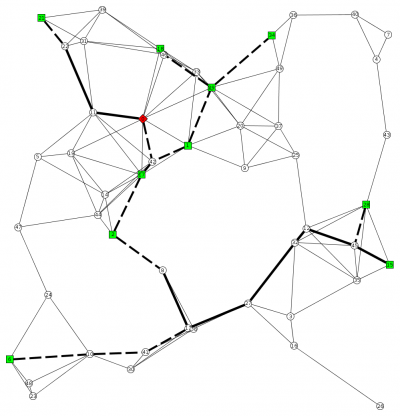
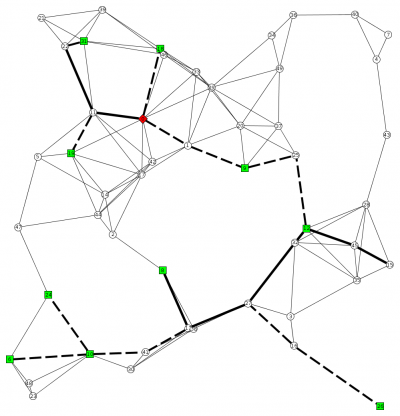
An optimum solution (1st and 3rd scenario) for an instance with 50 vertices and 5 scenarios is presented in the following pictures. The green vertices are the terminals in the scenario, the red vertex is the root node, the solid lines are the edges bought in the first stage, and the dashed lines the edges of the scenario.
As one can easily see, the first stage is disconnected and furthermore, in scenario 2 there are Steiner leaves.
The images are generated by storing the solution as .gml file, loading it with yEd, and exporting it as a .png.


